Featured images

[khyde]

Hello,

I was wondering if you could give some details on how some of the more recent true color Featured Images are created.  I have made some true color images in SeaDAS, but they don't look near as nice as the ones you featured in 2016 and 2017 with the strong contrast in the water colors.  Is there a tutorial on how to create images such as these?

Thanks,
Kim

[OB.DAAC - SeanBailey]

Kim,

Norman will probably respond, but likely not refer to it as magic...but I do :grin:
Way back in the distant past, Norman posted a "how-to" on one of his bits of SeaWiFS magic.
His magicians top hat has added more fairy dust over the years, but the the basics are there.
He also responded to a similar request on this forum that may also be of use to you.

Sean

[OB WebDev - norman]

Hi Kim,

The procedures I use to make the images that you may have seen vary a bit depending
on the scene in question, but there are some general similarities.  I'll share some of
the process that went into making the current feature image in case that helps.
The following bash script makes use of code from SeaDAS, the HDFGroup,
GMT, ImageMagick, pfstools, and Perl, plus some that I wrote myself which I will
attach to this message.  I will link to program descriptions where I can.

update_luts.py aqua

for f in A2017245125500; do
  wget https://oceandata.sci.gsfc.nasa.gov/cgi/getfile/$f.L1A_LAC.bz2
  bunzip2 $f.L1A_LAC.bz2
  modis_GEO.py $f.L1A_LAC
  getanc.py $f.L1A_LAC
  modis_L1B.py $f.L1A_LAC $f.GEO
  l2gen ifile=$f.L1B_LAC geofile=$f.GEO ofile=$f.L2_rhos_645 l2prod=rhos_645 resolution=250
  l2gen ifile=$f.L1B_LAC geofile=$f.GEO ofile=$f.L2_rhos_469_555_645 l2prod=rhos_469,rhos_555,rhos_645 resolution=500

  # Extract the pertinent data from the level-2 files.

  h5dump -d /geophysical_data/rhos_645 -b -o nak $f.L2_rhos_645
  cat nak >>rhos_645_q
  h5dump -d /navigation_data/latitude -b -o nak $f.L2_rhos_645
  cat nak >>lat
  h5dump -d /navigation_data/longitude -b -o nak $f.L2_rhos_645
  cat nak >>lon

  h5dump -d /geophysical_data/rhos_469 -b -o nak $f.L2_rhos_469_555_645
  cat nak >>rhos_469_h
  h5dump -d /geophysical_data/rhos_555 -b -o nak $f.L2_rhos_469_555_645
  cat nak >>rhos_555_h
  h5dump -d /geophysical_data/rhos_645 -b -o nak $f.L2_rhos_469_555_645
  cat nak >>rhos_645_h

done
rm nak

# Interpolate the 500-meter bands to 250-meter.
~/tools/bilinearmodis h q z rhos_469_h > rhos_469_hq
~/tools/bilinearmodis h q z rhos_555_h > rhos_555_hq
~/tools/bilinearmodis h q z rhos_645_h > rhos_645_hq

# Sharpen the blue and green bands using the red band as follows.
# Divide the interpolated blue (green) band by the quotient of the
# interpolated-250-meter red band over the native-250-meter red band.
# If either the native or interpolated red value is 0,
# then use a quotient of 1.
gmt math -bi1f -bo1f rhos_469_hq rhos_645_hq DUP rhos_645_q DUP 3 1 ROLL MUL 3 1 ROLL DIV 1 IFELSE DIV = rhos_469_q

gmt math -bi1f -bo1f rhos_555_hq rhos_645_hq DUP rhos_645_q DUP 3 1 ROLL MUL 3 1 ROLL DIV 1 IFELSE DIV = rhos_555_q

# Map the data.
f=A2017245125500
for i in rhos_???_q; do
    perl -e 'open X,"lon" or die;open Y,"lat" or die;open Z,"'$i'" or die;while(read(Z,$z,4)){read(X,$x,4);read(Y,$y,4);print $x,$y,$z}' | gmt mapproject -bi3f -bo3f -R3/-39/22/-23r -Jb13/-30/-34/-26/1:800000 | gmt nearneighbor -G$i.grd -I0.01 -N4 -R0/88.62/0/87.3 -S0.04 -r -bi3f -V
    gmt grdmath $i.grd 0.008 MAX 0.008 DIV LOG 2 0.008 DIV LOG DIV 1 MIN 65535 MUL = nak.grd
    gmt grd2xyz nak.grd -ZTLHw > nak.dat
    echo -e "P5\n8862 8730\n65535"|cat - nak.dat>$i.16bit.log.pgm
done

convert rhos_645_q.16bit.log.pgm rhos_555_q.16bit.log.pgm rhos_469_q.16bit.log.pgm -combine $f.rhos_645_555_469.log.tif
convert $f.rhos_645_555_469.log.tif -separate \( -clone 0 -equalize \) \( -clone 1 -equalize \) \( -clone 2 -equalize \) -delete 0-2 -combine $f.rhos_645_555_469.log.eq.png
pfsin $f.rhos_645_555_469.log.tif |pfstmo_fattal02 | pfsgamma 2.2| pfsout $f.rhos_645_555_469.log.fattal.png
pfsin $f.rhos_645_555_469.log.tif |pfstmo_mantiuk06 -e 0.5|pfsgamma 2.2|pfsout $f.rhos_645_555_469.log.mantiuk.png

# Make a chlorophyll map.
wget https://oceandata.sci.gsfc.nasa.gov/cgi/getfile/$f.L2_LAC_OC.nc
h5dump -d /geophysical_data/chlor_a -b -o chl A2017245125500.L2_LAC_OC.nc
h5dump -d /navigation_data/latitude -b -o lat A2017245125500.L2_LAC_OC.nc
h5dump -d /navigation_data/longitude -b -o lon A2017245125500.L2_LAC_OC.nc

perl -e 'open X,"lon" or die;open Y,"lat" or die;open Z,"chl" or die;$nd=pack "f",-32767;while(read(Z,$z,4)){read(X,$x,4);read(Y,$y,4);next if $z eq $nd;print $x,$y,$z}' | gmt mapproject -bi3f -bo3f -R3/-39/22/-23r -Jb13/-30/-34/-26/1:800000 | gmt nearneighbor -Gchl.grd -I0.01 -N4 -R0/88.62/0/87.3 -S0.12 -r -bi3f -V

gmt grdmath chl.grd 0.04 MAX 0.04 DIV LOG 20 0.04 DIV LOG DIV 1 MIN 65535 MUL = nak.grd
gmt grd2xyz nak.grd -ZTLHw > nak.dat
echo -e "P5\n8862 8730\n65535"|cat - nak.dat>chl.16bit.log.pgm

convert chl.16bit.log.pgm -fill gray -opaque black nak.tif
pfsin nak.tif|pfstmo_fattal02|pfsgamma 2.2|pfsout chl.fattal.png
pfsin nak.tif|pfstmo_mantiuk06 -e 0.5|pfsgamma 2.2|pfsout chl.mantiuk.png

So much for the semi-automated bulk of the work.  What I do next is load
the image layers I created above into my favorite image processing program,
the Gimp.  (You could also use any image software that can handle layers
such as Photoshop.  I just have become familiar with Gimp which has the
added advantage of being free.)  At this point it becomes harder to write
down a description since every image requires different blending techniques.
If you get this far, I would suggest that you experiment with different blending
operators to merge the layers.  The blending modes I use most often in Gimp are
overlay/soft light, screen, multiply, value, grain merge, and color.  I also make
liberal use of layer masks to control which portions of which layers get blended in.

It is also possible, of course, to blend layers in a non-interactive way using programs
such as those in the aforementioned ImageMagick suite, but it's much harder
to tailor blends to individual scenes without seeing how each layer affects the
result as it is being applied.

I hope you find this helpful.

Regards,
Norman

P.S.

One of my biggest challenges when working up images like these is sun glint
which obscures ocean color and accentuates sensor striping artifacts.  I would
be very pleased to have a sensor, like the ocean-color imager on the proposed
PACE mission, that tilts to avoid sun glint and avoids striping with a single-string
detector design.
attachment 1

[khyde]

Norman,

Thank you so much for your detailed description.  I'm hoping to get some time next week to try this out.

Kim

[dortenzio]

Good morning

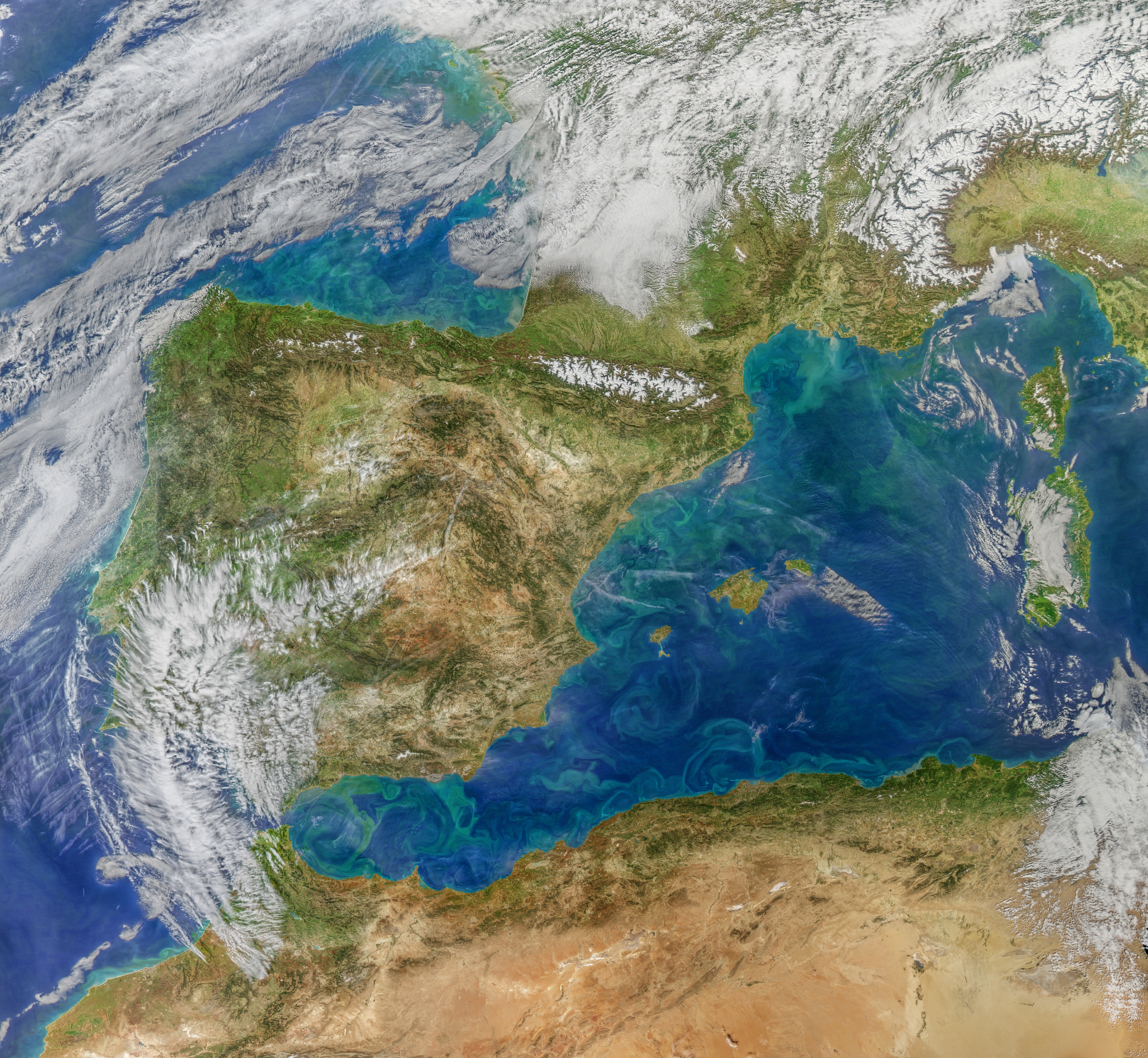
I resuscitated this post as a collegue of mine in Villefranche asked me if it was possible to reproduce (and possibly apply to other scenes) the « featured image » of the NW med visible in the OC web site https://oceancolor.gsfc.nasa.gov/feature/images/A2020071130500.WesternMed.jpg.
I then adapted the Norman script (in particular for the new wget and to solve a crash problem I experience in the gmt math apply to the bands). Anyway, for the most, the Norman script was incredibly well done.
I then try to initially reproduce the picture used as example in the 2017 Norman’s post https://oceancolor.gsfc.nasa.gov/cgi/image_archive.cgi?i=517.
The png results of the processing as well as my adapted script are here http://www.obs-vlfr.fr/~dortenzio/TrueColors/.

SO, my questions:

1. I’m not particularly satisfied of the generated png's. Chl pictures, in particular, seem badly interpolated, and I suspect, but in fact I have no idea, that the GMT nearneighbor et mapproject commands should be better parametrized. Have you any hints/suggestions??

2. Even considering that the generated png are ok (and I’m not sure, see previous point) the Gimp post processing is completely obscure for me. I used Gimp in a very basic way, so any suggestion to the use of gimp to obtain the aimed images from the series of png generated by the Norman scripts will be really appreciated.

Thank you so much for any help..and still congratulations for the excellent job at OC web site
Ciao
Fabrizio

[OB WebDev - norman]

Hi Fabrizio,

I looked at a couple of your images, and the moiré patterns indicate that the
chosen search radius passed to nearneighbor is too small for the spacing of
the projected input data.  A couple of possibilities spring to mind.

(a) I am not familiar with R.  Are you sure that your Rscript is outputting the data
      at the nominal 250-meter resolution?
(b)  When moving between map scales and image pixel dimensions, I think in terms
      of pixels (or dots) per inch.  I therefore find it easier to use GMT with
      PROJ_LENGTH_UNIT set to inch.  If any of your GMT calls are defaulting to
      centimeter, then you would need to adjust your mp scale and other parameters
      accordingly.  The map scale of 1:800000 when rendered at 100 dots per inch
      yields a pixel width of 800000*2.54/10000 = 203.2 meters.  This is smaller
      than the resolution of the sharpened MODIS data, but a search radius of -S0.04
      paired with a grid spacing of -I0.01 should be sufficient to avoid holes if the projected
      data are at least within 800 meters of each other.

With regards to gimp, I would suggest that you become familiar with working with image
layers, image-layer masks, and layer blending modes as well as the numerous tools and
filters (e.g. selection, air-brush, levels, curves, etc.).  There are many tutorials available
online.  Since I wrote my earlier post in this thread, I have also started using Gimp 2.10
which supports 16-bit image data.  If you have 2.10, you may want to consider saving
your intermediate products as TIFF instead of PNG to retain as much information as
possible during processing.

If you already know PhotoShop, you may consider using that program instead of gimp
since it has many of the same capabilities.

Regards,
Norman

[dortenzio]

Hi Norman

thank you very much for your rapid answer.
I delayed to repost, as my workstation crashed, and the containment laws in France avoid me to go to the lab to reboot it.. I had to ask to a colleague having a special permission to the servers rooms... what a period..
anyway..

(a) R script I create was relatively simple, just read, did basic operation and write output.. I obtained files at the right resolution..the true point was that it was extremely slow.. so, I preferred to install the last version of GMT, and I now used your old code.

(b) yes, my PROJ_LENGTH_UNIT was in cm, so all the parameters was wrongly defined. Great.

(c) I still slightly modified your code to more easily modify resolution of outputs.

Resulting images and present script are still here http://www.obs-vlfr.fr/~dortenzio/TrueColors/

By the way...I’m not sure about results.

1) Chl png seems ok, although I still have problems to understand how apply palette under gimp (why do you prefer to generate a B&W picture?? Gimps palette seems awful .. probably I miss some easily process in gimps) .

2) on the other hand, png of bands seem still not rightly processed..or maybe I miss some passages. I should at least recognize some patterns in the A2017245125500.rhos_645_555_469.log.mantiuk scene... but it seems complete badly processed..

again, any helps should be really appreciated
thank you again
ciao
Fabrizio

[OB WebDev - norman]

Hi Fabrizio,

We have the same issues accessing our work place at Goddard Space Flight Center in
Maryland.  Yes, these are challenging times.

There is still something wrong with the files you are generating.  They should not
have those holes in the grid.  I notice that you have many key lines commented out
in your most recent script.  Are you sure you are updating all your intermediate files?

I run my scripts on a linux box that uses little-endian byte ordering.  Therefore,
I swap bytes when writing out 16-bit PGM files so as to follow the de facto standard
to write the most significant byte first.  If you are already on a big-endian machine
then you may want to try replacing "-ZTLHw" with "-ZTLH" in the grd2xyz call.

I can't think of anything else at the moment.

Norman

P.S.
You do not need to repeat the gmt for commands that start with "gmt".
So, for example, you can just say "gmt set PROJ_LENGTH_UNIT inch".

Also, in case you wondered, the file names that begin with "nak" are just
temporary files that I named using my initials.

[OB WebDev - norman]

Oh, with regards to your comment about applying a palette under gimp: I do not
use the chlorophyll images in that way i.e. as indexed color look-up tables.  I blend
the gray-scale chlorophyll images with the other layers using blending modes such
as "soft light".  That particular blending mode has the effect of brightening or darkening
pixels in the underlying layers depending on whether the chlorophyll pixels are
greater than or less than 50% gray, respectively.  I like to use this technique to
enhance color gradients.

Norman

[dortenzio]

Dear Norman

thanks again!!
as you suspected, most of the intermediate files were corrupted.
By relaunching the whole script, I obtained finally good results. I slightly reduced the resolution to better manage the remote processing due to confinement (I have good connection at home, but network is completely saturated ).
Images are here: http://www.obs-vlfr.fr/~dortenzio/TrueColors/small/

I have now to deal with gimp, and even with your tips, I have still several difficulties to obtain « nice » pictures (I’m not used with mouse based interface.. I prefer old style command based procedures). For example, blending Chl/log with RRs_log images through « soft-light » blending mode of gimp (as you suggested), produces some results, but colorization of the « ocean » portion of the image rests still incomplete. I have to definitively ameliorate my skills with gimp.

Anyway,  I read that Image Magick could reproduce most of the features of Gimp in a script, so my objective now is to try to understand how blend the different layers with gimp and, even if the results will be not so nice as yours, try to generate automatically that kind of pictures.
In some way, I am  ready to accept less nice images to produce time series of true color pictures.

Thank you again for your help
And If you have still some suggestions, I will really appreciate
Fabrizio