Hello,
I am trying to screen the extinction coefficient profiles from CALIPSO data (CAL_LID_L2_05kmAPro-Standard-V4) based on CAD score (CAD score>-20) and plot it vs altitude (https://hdfeos.org/zoo/MORE/LaRC/CALIPSO/CAL_LID_L2_05kmAPro-Standard-V4-21.2021-01-10T21-34-11ZN.hdf.py.png). I took help from https://www-calipso.larc.nasa.gov/resources/calipso_users_guide/tools/files/Generate_Mean_Extinction_Profile_v3.pdf but this is in MATLAB. I am unable to do it in python.
Can anyone help me with this.
Thanks.
Screening the CALIPSO aerosol profiles based on CAD score
-
ASDC - cheyenne.e.land
- Subject Matter Expert

- Posts: 131
- Joined: Mon Mar 22, 2021 3:55 pm America/New_York
- Has thanked: 1 time
- Been thanked: 8 times
Re: Screening the CALIPSO aerosol profiles based on CAD score
Hello,
Thank you for your interest in CALIPSO data.
We're currently working on python code to get you what you need. Thank you for your patience.
Regards,
ASDC
Thank you for your interest in CALIPSO data.
We're currently working on python code to get you what you need. Thank you for your patience.
Regards,
ASDC
-
ASDC - cheyenne.e.land
- Subject Matter Expert
- Posts: 131
- Joined: Mon Mar 22, 2021 3:55 pm America/New_York
- Has thanked: 1 time
- Been thanked: 8 times
Re: Screening the CALIPSO aerosol profiles based on CAD score
Hello,
We used code made by HDF-EOS that graphs the Extinction Coefficient v Altitude and revised it to only plot values based on the CAD Score greater than -20.
Here is what output graph should look like:
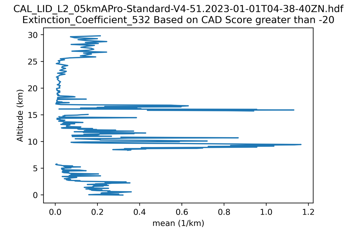
Update: Had to make a quick revision to the code due to an error. Above is the new image.
We used code made by HDF-EOS that graphs the Extinction Coefficient v Altitude and revised it to only plot values based on the CAD Score greater than -20.
Code: Select all
import os
import numpy as np
import matplotlib as mpl
import matplotlib.pyplot as plt
from pyhdf import HDF, SD, VS
from pyhdf.SD import SD, SDC

FILE_NAME = 'CAL_LID_L2_05kmAPro-Standard-V4-51.2023-01-01T04-38-40ZN.hdf'
DATAFIELD_NAME = 'Extinction_Coefficient_532'
cad_score = 'CAD_Score'
sd = SD(FILE_NAME, SDC.READ)
hdf = HDF.HDF(FILE_NAME)
vs = hdf.vstart()

xid = vs.find('metadata')
altid = vs.attach(xid)
altid.setfields('Lidar_Data_Altitudes')
nrecs, _, _, _, _ = altid.inquire()
altitude = altid.read(nRec=nrecs)
altid.detach()
alt = np.array(altitude[0][0])

# Read dataset.
data2D = sd.select(DATAFIELD_NAME)
data2D_cad = sd.select(cad_score)

# Read attributes.
attrs = data2D.attributes(full=1)
attrs_cad = data2D_cad.attributes(full=1)
fva=attrs["fillvalue"]
fva_cad=attrs_cad["fillvalue"]
fillvalue = fva[0]
fillvalue_cad = fva_cad[0]
ua=attrs["units"]
units = ua[0]
vra=attrs["valid_range"]
valid_range = vra[0].split('...')

# Note: CAD_Score is a 3-D array of the size [#profiles, # altitude bins, 2].
#The first dimension, [ : , : , 0], corresponds to the standard altitude array of the Profile Products.
#Thus, below 8.3 km, the first dimension contains the descriptive flags of the higher of the two full resolution
#(30 m) bins that comprise the single 60 m bin reported in the Profile Products.
#Meanwhile, below 8.3 km, the second dimension [: , : , 1] contains the descriptive flags for the lower of the two
#30 m range bins. Above 8.3 km, where the range resolution of the Level 1 data is 60 m or greater,
#the descriptive flags for each single 60 m (or 180 m) range bin are replicated in both array elements.

data = data2D[:,:]
data_cad = data2D_cad[:,:,0]

# Filter fill value and valid range. See Table 66 (p. 116) from [1]
data[data == fillvalue] = np.nan
data_cad = data_cad.astype('float')
data_cad[data_cad == fillvalue_cad] = np.nan

#Filter CAD_Score to get only values greater than -20
data_cad[data_cad <= -20] = np.nan

#Filter Extinction_Coefficient_532 based on CAD_Score greater than -20
data[np.isnan(data_cad)] = np.nan


# Apply the valid_range attribute.
invalid = np.logical_or(data < float(valid_range[0]),
                        data > float(valid_range[1]))
data[invalid] = np.nan
datam = np.ma.masked_array(data, mask=np.isnan(data))
datam = np.mean(datam, axis=0)
vs.end()
sd.end()

plt.plot(datam, alt)
plt.ylabel('Altitude (km)')
title = 'Extinction_Coefficient_532 Based on CAD Score greater than -20'
basename = os.path.basename(FILE_NAME)
plt.xlabel('{0} ({1})'.format('mean', units))
plt.title('{0}\n{1}'.format(basename, title))
fig = plt.gcf()
pngfile = "{0}.py.png".format(basename)

fig.savefig(pngfile, dpi=400)

# Reference
# [1] https://www-calipso.larc.nasa.gov/products/CALIPSO_DPC_Rev4x92.pdf
Update: Had to make a quick revision to the code due to an error. Above is the new image.